Basic controls
Once a Jupyter or Qt widget has been created, the way in which you change settings and interact with WorldWide Telescope is the same.
Visual settings
Once the WorldWide Telescope Jupyter or Qt widget has been initialized – here
we assign it to the variable name wwt – you can toggle several visual
settings on and off. For example:
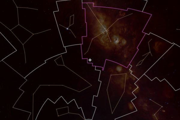
>>> wwt.constellation_boundaries = True
shows the boundaries of the formally defined regions for each constellation. You can show the constellations themselves by changing another setting:
>>> wwt.constellation_figures = True
These two settings and constellation_selection also have complementary
settings that change their colors. These settings take either color names,
string hex codes, tuples of (red, green, blue) values (where each value
should be in the range [0:1]) tuples or more generally anything recognized
by the matplotlib.colors.to_hex() function from Matplotlib:
>>> wwt.constellation_boundary_color = 'azure'
>>> wwt.constellation_figure_color = '#D3BC8D'
>>> wwt.constellation_selection_color = (1, 0, 1)
Numerical settings all take values as Astropy astropy.units.Quantity
objects, which are floating point values with associated units. To demonstrate
this, let’s say you’d like to simulate the celestial view from the top of the
tallest building in Santiago, Chile. You would then enter:
>>> from astropy import units as u
>>> wwt.local_horizon_mode = True
>>> wwt.location_latitude = -33.4172 * u.deg
>>> wwt.location_longitude = -70.604 * u.deg
>>> wwt.location_altitude = 300 * u.meter
All of the preceding code results in the following view:
If you are using the Qt widget, you can save a screenshot like the one above through a method that takes your desired file name its argument:
>>> wwt.render('stgo_view.png')
Centering on coordinates
While you can click and drag to pan around and use scrolling to zoom in and out,
it’s also possible to programmatically center the view on a particular object or
region of the sky, given a certain set of coordinates in the form of an astropy
SkyCoord object and a field of view (zoom level in
astropy pixel units) for the viewer. You can read more about creating
SkyCoord objects here. One of the useful
features of this class is the ability to create coordinates based on an object
name, so we can use this here to center on a particular object:
>>> from astropy import units as u
>>> from astropy.coordinates import SkyCoord
>>> coord = SkyCoord.from_name('Alpha Centauri')
>>> wwt.center_on_coordinates(coord, fov=10 * u.deg)
Foreground/background layers
Up to two image layers can be shown in the viewer. The viewer’s ability to display multiple layers allows users to visually compare large all-sky surveys and smaller studies. They can also add a good amount of aesthetic value for tours or general use, and there are several methods of selecting them.
About 20 layers of different wavelengths, scopes, and eras are currently
available. You can list them using the widget’s
available_layers attribute:
>>> wwt.available_layers
['2MASS: Catalog (Synthetic, Near Infrared)', '2Mass: Imagery (Infrared)',
 'Black Sky Background', 'Digitized Sky Survey (Color)',
 'Fermi LAT 8-year (gamma)', 'GALEX (Ultraviolet)', 'GALEX 4 Far-UV',
 'GALEX 4 Near-UV', 'Hydrogen Alpha Full Sky Map',
 'IRIS: Improved Reprocessing of IRAS Survey (Infrared)',
 'Planck CMB', 'Planck Dust & Gas', 'RASS: ROSAT All Sky Survey (X-ray)',
 'SDSS: Sloan Digital Sky Survey (Optical)', 'SFD Dust Map (Infrared)',
 'Tycho (Synthetic, Optical)',
 'USNOB: US Naval Observatory B 1.0 (Synthetic, Optical)',
 'VLSS: VLA Low-frequency Sky Survey (Radio)', 'WISE All Sky (Infrared)',
 'WMAP ILC 5-Year Cosmic Microwave Background']
Using the foreground and background attributes, it is possible to
directly set layers using these full names. The opacity of the foreground layer
is also modifiable:
>>> wwt.background = 'Fermi LAT 8-year (gamma)'
>>> wwt.foreground = 'Planck Dust & Gas'
>>> wwt.foreground_opacity = .75
For easier layer assignment, especially when you don’t yet know which layer you
want, use the imagery attribute. It automatically sorts layers by
wavelength (‘radio’, ‘uv’, etc.), shortens their names, and allows for their
selection through tab completion. The resulting objects point back to the
original layer names, so they can be used in the same manner as above:
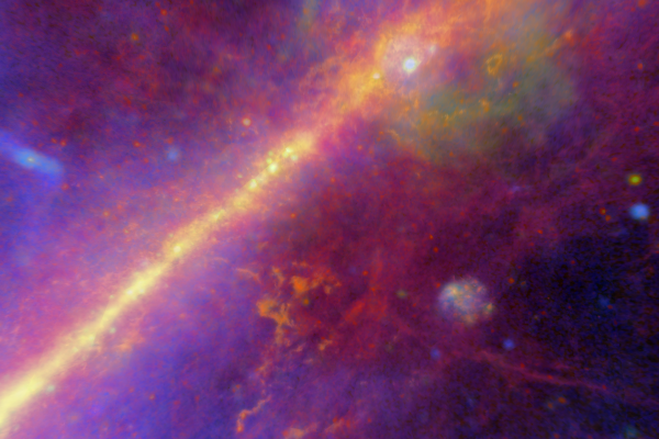
>>> wwt.background = wwt.imagery.gamma.fermi
>>> wwt.foreground = wwt.imagery.other.planck
>>> wwt.foreground_opacity = .75
The preceding code superimposes a dust and gas map on an all-sky gamma ray intensity survey and produces the following output:
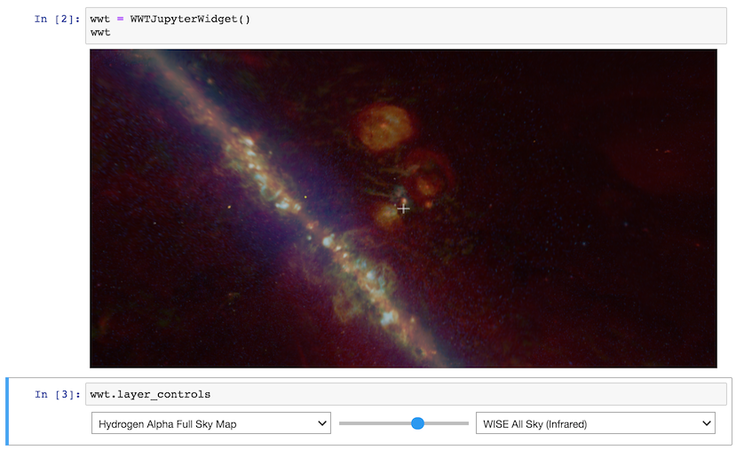
In the Jupyter version, it is possible to add GUI controls that allow the layers to be chosen from drop down menus. To get these, type:
>>> wwt.layer_controls
The controls also include a slider that interactively changes the opacity of the foreground layer, as shown in the following image: