Adding data layers
While annotations (see Showing annotations) can be used to show specific points of interest on the sky, data layers are a more general and efficient way of showing point-based data anywhere in 3D space, including but not limited to positions on the sky and on/around celestial bodies. In addition, layers can be used to show image-based data on the celestial sphere.
The main layer type for point-data at the moment is
TableLayer. This layer type can be created using an
astropy
Table as well as a coordinate frame, which can be e.g.
'Sky' or the name of one of the planets or satellites. The main layer type
for images is ImageLayer.
Loading point data
To start off, let’s look at how to show a simple set positions on the sky. We’ll use the Open Exoplanet Catalogue as a first example. We start off by using astropy.table to read in a comma-separated values (CSV) file of the data:
>>> from astropy.table import Table
>>> OEC = 'https://worldwidetelescope.github.io/pywwt/data/open_exoplanet_catalogue.csv'
>>> table = Table.read(OEC, delimiter=',', format='ascii.basic')
Assuming that you already have either the Qt or Jupyter version of pywwt open
as the wwt variable, you can then do:
>>> wwt.layers.add_table_layer(table=table, frame='Sky',
...                            lon_att='ra', lat_att='dec')
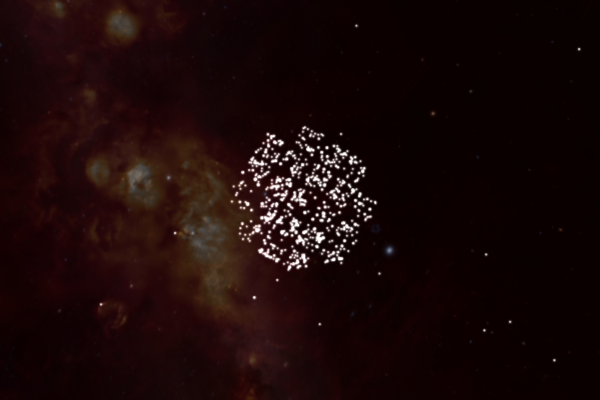
Note that we have specified which columns to use for the right ascension and
declination (in the Sky frame, lon refers to right ascension, and
lat to declination).
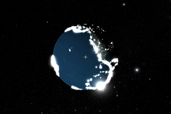
Let’s now look at how to load data in the frame of reference of a celestial body. Let’s first change the camera settings so that we are looking at the Earth (see Changing and controlling views for more details):
>>> wwt.set_view('solar system')
>>> wwt.solar_system.track_object('Earth')
Be sure to zoom in so that you can see the Earth properly. Next, we use a dataset that includes all recorded earthquakes in 2010:
>>> from astropy.table import Table
>>> EARTHQUAKES = 'https://worldwidetelescope.github.io/pywwt/data/earthquakes_2010.csv'
>>> table = Table.read(EARTHQUAKES, delimiter=',', format='ascii.basic')
We can then add the data layer using:
>>> layer = wwt.layers.add_table_layer(table=table, frame='Earth',
...                                    lon_att='longitude', lat_att='latitude')
Note that lon_att and lat_att don’t need to be specified in
add_table_layer - they can also be set
afterwards using e.g.:
>>> layer.lon_att = 'longitude'
In some cases, datasets provide a third dimension that can be used as an
altitude or a radius. This can be provided using the alt_att column:
>>> layer.alt_att = 'depth'
Using cartesian coordinates
In some cases, you may instead want to load data in cartesian coordinates. In
this case, you will need to set coord_type='rectangular' and use x_att,
y_att, and z_att to set the columns to use for the x/y/z positions:
>>> layer.coord_type = 'rectangular'
>>> layer.x_att = 'x_kpc'
>>> layer.y_att = 'y_kpc'
>>> layer.z_att = 'z_kpc'
and the unit for the coordinates can be set with:
>>> layer.xyz_unit = 'au'
Editing data settings
There are several settings that can be used to fine-tune the interpretation of the data. First, we can set how to interpret the ‘altitude’:
>>> layer.alt_type = 'distance'
The valid options are 'distance' (distance from the origin), altitude
(outward distance from the planetary surface), depth (inward distance from
the planetary surface), and sealevel (reset altitude to be at sea level).
It is also possible to specify the units to use for the altitude:
>>> from astropy import units as u
>>> layer.alt_unit = u.km
This should be an astropy Unit and should be one of
u.m, u.km, u.au, u.lyr, u.pc, u.Mpc,
u.imperial.foot, or u.imperial.mile. It is also possible to pass a
string provided that when passed to Unit this returns
one of the valid units.
Finally, it is possible to set the units for the longitude:
>>> layer.lon_unit = u.hourangle
The valid values are u.degree and u.hourangle (or simply u.hour) or
their string equivalents.
Enabling time series attributes
If your table has a column of times, you can animate your data by activating the time series attribute and specifying the proper column:
>>> layer.time_series = True
>>> layer.time_att = 'time'
(Please note that time columns must contain
astropy
Time objects, datetime objects, or
ISOT compliant strings.)
Once the time in the viewer matches an object’s stated time in the table, its corresponding point will pop into view. See Changing and controlling views for more information on how to control time in the viewer.
By default, time series points disappear 16 days (viewer time, not necessarily
real time) after they pop up. You can adjust their decay time using Quantity objects:
>>> layer.time_decay = 2 * u.hour
To allow time series-enabled points to remain visible forever after they first
appear, set time_decay equal to zero (still
remembering to use units).
Note
Limitations of WWT’s current date calculation algorithm for time series layers cause decreasing precision in displaying points as their dates move away from 2010. For a year like 2019, points within a few seconds of each other appear simultaneously. The same is true for points within a minute of each other for a year like 2110. Points with offsets on the order of days or more are largely unaffected.
Choosing visual attributes
There are a number of settings to control the visual appearance of a layer. First off, the points can be made larger or smaller by changing:
>>> layer.size_scale = 10.
It is also possible to make the size of the points depend on one of the columns
in the table. This can be done by making use of the size_att attribute:
>>> layer.size_att = 'mag'
then using layer.size_vmin and layer.size_vmax to control the values
that should be used for the smallest to largest point size respectively.
Similarly, the color of the points can either be set as a uniform color:
>>> layer.color = 'red'
or it can be set to be dependent on one of the columns with:
>>> layer.cmap_att = 'depth'
then using layer.cmap_vmin and layer.cmap_vmax to control the values
that should be used for the colors on each end of the colormap. By default
the colormap is set to the Matplotlib ‘viridis’ colormap but this can be changed
using the following attribute, which should be given the name of a Matplotlib
colormap
or a colormap object:
>>> layer.cmap = 'plasma'
By default, the marker size stays constant relative to the screen, but this can be changed with:
>>> layer.marker_scale = 'world'
To change it back to be relative to the screen, you can do:
>>> layer.marker_scale = 'screen'
Finally, if you want to show all markers even if they are on the far side of a celestial object, you can use:
>>> layer.far_side_visible = True
Image layers
Image layers are added in a similar way to point data, using
add_image_layer:
>>> layer = wwt.layers.add_image_layer(image='my_image.fits')
Here, the image input can be either a filename, an
ImageHDU object, or a tuple of the form
(array, wcs) where array is a 2-d Numpy array, and wcs is an
astropy WCS object. Once the image has loaded,
you can modify the limits, stretch, and opacity using:
>>> layer.vmin = -10
>>> layer.vmax = 20
>>> layer.stretch = 'log'
>>> layer.opacity = 0.5
Listing and removing layers
You can list the layers present in the visualization by doing:
>>> wwt.layers
Layer manager with 1 layers:

  [0]: TableLayer with 1616 markers
You can remove a layer by either doing:
>>> layer.remove()
or:
>>> wwt.layers.remove_layer(layer)
If you don’t have a reference to the layer, you can always do:
>>> wwt.layers.remove_layer(wwt.layers[0])